As mentioned last time, I am going to cover different types of graphs
Pie charts vs. bar charts:

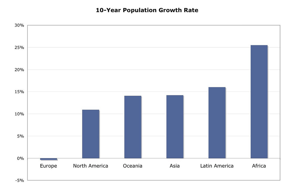
Bar graphs are another type of data visualization which most people have seen. It is where the data is represented as bars, where the x-axis is the independent variable, and the y-axis is the dependent variable.
Pie charts have the advantages of displaying categories within one set with respect to one another and being used best with percentages. They have the disadvantages of needing each category displayed to be read correctly (no truncation) and that all data values must be present. Bar charts have the advantages of being very flexible (there is no distortions from truncating categories) and they can compare 2 or more data sets. The disadvantage is that it is not very useful for percentages.
Stem-and-Leaf plot vs. histogram.
Stem and Leaf plots are those graphs which show the non-ones-place as the stem and the ones place as the leaves. What you do is put the stems on one column, and the leaves of the corresponding data points next to their appropriate stems. Since there is no way to explain it well without an example, I'll use a picture.
 |
| The low is 20 and the high is 102. |
Histograms are a special type of bar graphs. Each bar represent a range of x-values (independent variables) and the height represents the frequency between the two x-values.

For stem-and-leaf plots, the only advantage is that each data point is seen in the graph. The cons is that it is inflexible and not suitable for a large range of data points. Histograms are very flexible, good to see the theoretical distribution, and useful for spotting outliers. The only con is that is cannot see individual data points. Histograms are used to show frequency of data points within a given interval.
Scatter Plot vs. Line Graph:
A scatter plot puts a dot at each x-y pair, where x is the independent variable and y is the dependent variable. This is the most common graph type when performing statistical regression analysis.

Line graphs are where there is only one data point corresponding to each x point. It's similar to a scatter plot, but each point represents the average of y-values.

The advantage to a scatter plot is that it shows all data points and we can see a general trend if one is to be found. We can also see how strong the trend is. The disadvantage is that it can get exceedingly cluttered exceedingly quickly, and it is not practical to look at each data point individually. Line graphs have the advantage of being much easier to look at each individual point readily. The disadvantage is that it does not display each data point, just the average of y values at a given x value.
These are the common types of non-probability graphs of data used in statistics. Next time, I'll be covering a more detailed look into data sets. Until then, stay curious.
K. "Alan" Eister has his bacholers of Science in Chemistry. He is also a tutor for Varsity Tutors. If you feel you need any further help on any of the topics covered, you can sign up for tutoring sessions here.
K. "Alan" Eister has his bacholers of Science in Chemistry. He is also a tutor for Varsity Tutors. If you feel you need any further help on any of the topics covered, you can sign up for tutoring sessions here.
Comments
Post a Comment