Basic Statistics Lecture #3: Normal, Binomial, and Poisson Distributions

As I have mentioned last time, the uniform continuous distribution is not the only form of continuous distribution in statistics.  As promised, here are the three most common continuous distribution types.  As a side note, all sampling distributions are relative to the algebraic mean.

Normal Distribution:

I think most people are familiar with the concept of a normal distribution.  If you've ever seen a bell curve, you've seen the normal distribution.  If you've begun from the first lecture of this lecture series, you've also seen the normal distribution.

This type of distribution is where the data points follow a continuous curve, is non-uniform, has a mean (algebraic average) equal to the median (the exact middle value), falls from highest probability at the mean to (for all practical purposes) zero as the x-values approach $\pm \infty$, and therefor has equal number of data points to the left and to the right of the mean, and has the domain of $(\pm \infty)$, and a range of $(0, P(\bar{x})]$.  This is a well-observed type of distribution.  Take the probability of a value with rolling dice as an example.  Rolling one die has a uniform discrete probability.  Rolling two dice has a discrete probability distribution which is reminiscent of the continuous normal distribution curve.  Go to three dice and the continuous normal distribution.  The more dice you add, the closer we get to a continuous normal distribution curve.  So this is an observed phenomenon.  In fact, regardless of whether the distribution type is discrete or continuous, regardless of whether they are uniform, normal, random, chi-squared, Poisson, or any other type, all distributions are derived from observation, not from mathematical proof.

For those of you who are curious, the normal distribution is bound by the x axis and the bell shaped curve of the form $\frac{1}{\sqrt{2\pi \sigma ^{2}}} \cdot e^{-\frac{(x-\mu )}{\sigma^2}}$, where the sigma-squared is the variance (square of the standard deviation) of the population, pi is the 3.141592 we all know so well, x is the mean of the sample we are looking at, and mu is the proposed mean of the population as a whole.  For example, the baseball season just ended.  The average ERA of the starting pitchers of the 8 teams who made it to the Division Series would be the value for x, the average ERA of starting pitchers of all 30 teams would be the value for mu, and the square of the standard deviation of the ERA of starting pitchers of all 30 teams is the value for sigma-squared.

Binomial Distribution:
Less well known is the binomial distribution.  In this type of distribution, there are only two outcomes, such as a heads or tails, or water falling from the sky or water not falling from the sky.

This is technically a type of discrete probability for any sample of size less than the population size, but as that size grows to the population size, the model approaches a continuous distribution.  Whether the mean equals the median depends on the difference between the two probabilities.  If there is a 50%-50% split, than they are equal.  Otherwise, they are not, and the greater the separation between the two probabilities, the greater the difference between the mean and the median.  It's domain is $[0, 1]$ while it's range is $[0, P(\bar{x})]$.

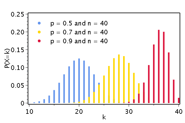
The distribution of the probabilities in the binomial distribution model of a sample is given by $ _{n}\textrm{P}_{x} =\tfrac{n!} {(n-x)!} \times p^n \times(1-p)^x$, where n is the sample size, x is the number of times in the sample of the event called successes, and p is the probability of said event.

Poisson Distribution:
Even lesser known than the binomial distribution is the Poisson distribution.  As a side note, it is not called Poisson because it is poisonous, but rather this distribution was introduced to the European masses by a guy named Siméon Denis Poisson.

Yeah, this guy is Poissonous.

He discovered that when the domain of the normal distribution has a minimum value of zero and the x axis represents the number of occurrences instead of a value of the system, its mean (point on the domain with the highest probability of occurring) is skewed towards the zero point in the domain, and drops to zero as the z-coordinate gets higher.  The number of occurrences can be the number of wins a baseball team has or the number of pitches a pitcher goes through before being pulled from the game, or anything countable.  He also, noticed that the higher the mean is, the lower the probability of the mean number of events, given by the Greek letter $\lambda$.

The curve which describes the Poisson distribution is given by $P(X=k)=\frac{\lambda ^{k}e^{- \lambda}}{k!}$, where k is the value of interest (120 pitches, for example), $\lambda$ is the "expectation value" of average of the distribution (102 pitches on average for starters, for example), and e is Euler's number 2.71828.

So those are the three most common continuous distributions.  If you have any questions, please post a comment.  Next time, I will begin the probability side of the course.  Until then, stay curious.

---

K. "Alan" Eister has his bacholers of Science in Chemistry. He is also a tutor for Varsity Tutors.  If you feel you need any further help on any of the topics covered, you can sign up for tutoring sessions here.