As promised last time, this lecture introduces the concept of Probability Theory. This is necessary to all statistical calculation. After all, statistical analysis depends on the concept of probability in order to get to the statistics, especially when we start dealing with regression analysis and analysis of variance (ANOVA).
The concept of probability deals with Venn diagrams. For those of you who don't know, Venn diagrams are those diagrams which lets us easily represent which elements two (or more) sets have in common and which elements they don't have in common.
 |
| Seems about right. |
So yes, they can be used to analyze costs. And the intersection of physical systems. In fact, they can be utilized to analyze almost any type of system. I'm currently using venn diagrams to analyze known conspiracies such as the Tuskegee Syphilis Experiment, the NSA spying scandal, and the governments' poisoning of the alcohol supply during Prohibition, all in order to check the statistical probabilities of supposed conspiracies, such as vaccines, Global Climate Change, and the False History hypothesis.
To start off, we have the general two-set Venn diagram, where the two sets are denoted by A and B. Because, you know, first two letters of the Latin alphabet.
 |
| Venn Diagram 1: Two variables (Not Mutually Exclusive) |
Mutually exclusive events are two events A and B which share no sample points. Generally speaking, this is where event A and event B have no baring on one another. This stems the theorem which states that if A and B are mutually exclusive, then their probabilities, taken together, is given by
$$P(A \vee B)=P(A)+P(B).$$
$$P(A \vee B)=P(A)+P(B).$$
 |
| Venn Diagram 2: Two mutually exclusive variables A and B. |
If they are not mutually exclusive (as in Venn Diagram 1), then
$$P(A \vee B)=P(A)+P(B)-P(A \wedge B)$$
If they are mutually exclusive (as in Venn Diagram 2), then
$$P(A \wedge B)=0$, so $P(A \vee B)=P(A)+P(B)-0=P(A)+P(B)$$
The down-carrot is the symbolic logic notation for the word "or", which (in probability) is an "exclusive or", which means either case but not both. The up carrot is the symbol for the word "and", which means both, but not either separately. The downward facing U $\cap$ is the intersect between the two sets, $A \cup B = A \vee B$. The upwards-facing $\cup$ (read as Union, as in AUB=A union B) is conceptually either A alone or B alone or both A and B $A \cap B$.
As a side note: these equations are never NOT true. Independence cannot be determined exclusively by looking at a sample space. Two events A and B are independent if and only if P(A∧B)=P(A)⋅P(B).
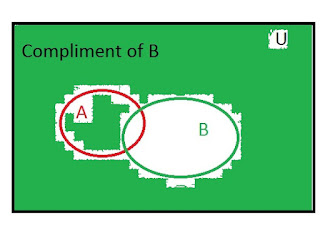
There are situations where we want to look at what's outside of the data sets. We call this situation the "compliment" of the set. For what's outside of set A, we call that A-compliment, which is written as $A^{c}$. The same applies for set B; the compliment of B is given by $B^{c}$.
 |
| $A^{c}$ is everything outside of A, regardless of whether or not it's outside of B. |
 |
| $B^{c}$ is everything outside of B, regardless of whether or not it's outside of A. |
 |
| $B^{c} \cup A^{c}$, everything outside of both A and B. |
 |
| $B^{c} \cap A^{c}$, everything which is either outside A or outside of B. |
Notice that the compliment of A or the compliment of B contains everything except the overlap between the two. If they were independent events, then there would be no overlap, so that $B^{c} \cap A^{c}$ would contain everything in the system. For this reason, the probability of $B^{c} \cap A^{c}$ will always be one if and only if A and B are independent sets.
Conditional Probability happens in non-Independence situations and have the conditional probability of $P(A∣B)=\frac {P(A∧B)}{P(B)}$. [P(A|B) is read “the probability of A given B”]. Note: Independence is where the probabilities of A and B do NOT affect one another. Conditional probability is where the probabilities of A and B DO affect one another. That the probability of A given B is saying is equivalent to "I want to choose B, so I am guaranteed to get B. Therefor, we need to mathematically make the probability of B equivalent to 100% in this case" We do that by putting it in the denominator of the calculation.
 |
| Venn Diagram 9: $B^{c} \cap A^{c}$ will always contain everything when A and B are completely independent sets. |
That ends the introduction to probability. If you have any questions, please leave a comment. Next time, I will cover Baye's Theorem. Until then, stay curious.
K. "Alan" Eister has his bacholers of Science in Chemistry. He is also a tutor for Varsity Tutors. If you feel you need any further help on any of the topics covered, you can sign up for tutoring sessions here.
Comments
Post a Comment